Introduction

I last left chapter 2 of Maching Learning for Hackers (a long time ago), running some kernel density estimators on height and weight data (see here. The next part of the chapter plots a scatterplot of weight vs. height and runs a lowess smoother through it. I’m not going to write any more about the lowess function in statsmodels. I’ve discussed some issues with it (i.e. it’s slow) here. And it’s my sense that the lowess API, as it is now in statsmodels, is not long for this world. The code is all in the IPython notebooks in the Github repo and is pretty straightforward.

Patsy and statsmodels formulas

What I want to skip to here is the logistic regressions the authors run to close out the chapter. Back in the spring, I coded up the chapter in this notebook. At this point, there wasn’t really much cohesion between pandas and statsmodels. You’d end up doing data exploration and munging with pandas, then pulling what you needed out of dataframes into numpy arrays, and passing those arrays to statsmodels. (After writing seemingly needless boilerplate code like X = sm.add_constant(X, prepend = True). Who’s out there running all these regressions without constant terms, such that it makes sense to force the use to explicitly add a constant vector to the data matrix?)

Over the summer, though, something quite cool happened. patsy brought a formula interface to Python, and it got integrated into a number components of statsmodels. Skipper Seabold’s Pydata presentation is a good overview and demo. In a nutshell, statsmodels now talks to your pandas dataframes via an expressive “formula” description of your model.

For example, imagine we had a dataframe, df, with variables x1, x2, and y. If we wanted to regress y on x1 and x2 with the standard statmodels API, we’d code something like the following:

Xmat = sm.add_constant(df[['x1', 'x2']].values, prepend = True)
yvec = df['y'].values
ols_model = OLS(yvec, Xmat).fit()

Which is tolerable with short variable names. Once you start using longer names or need more RHS variables it becomes a mess. With patsy and the formula API, you just have:

ols_model = ols('y \~ x1 + x2', df = df).fit()

Which is just as simple as using lm in R. You can also specify variable transformations and interactions in the formula, without needing to pre-compute variable for them. It’s pretty slick.

All of this is still brand new, and largely undocumented, so proceed with caution. But I’ve gotten very excited incorporating it into my code. Stuff I wrote just 5 or 6 months ago looks clunky and outdated.

So I’ve updated the IPython notebook for chapter 2, here, to incorporate the formula API. That’s what I’ll discuss in the rest of the post.

Logistic regression with formulas in statmodels

The authors run a logistic regression to see if they can use a person’s height and weight to determine their gender. I’m not really sure why you’d run such a model (or how meaningful it is once you run it, given how co-linear height and weight are), but it’s easy enough for illustrating how to mechanically run a logistic regression and use it to linearly separate groups.

The dataset contains variables Height, Weight, and Gender. The latter is a string encoded either Male or Female. To run a logistic regression, we’ll want to transform this to a numerical 0/1 variable. We can do this a number of ways, but I’ll use the map method.

heights_weights['Male'] = heights_weights['Gender'].map({'Male': 1, 'Female': 0})

The statstmodels.formula.api module has a number of functions, including ols, logit, and glm. If we import logit from the module we can run a logistic regression easily.

male_logit = logit(formula = 'Male \~ Height + Weight', df = heights_weights).fit()
print male_logit.summary()

With these results:

Optimization terminated successfully.
Current function value: 2091.297971
Iterations 8
Logit Regression Results

==============================================================================
Dep. Variable: Male No. Observations: 10000
Model: Logit Df Residuals: 9997
Method: MLE Df Model: 2
Date: Thu, 20 Dec 2012 Pseudo R-squ.: 0.6983
Time: 14:41:33 Log-Likelihood: -2091.3
converged: True LL-Null: -6931.5
LLR p-value: 0.000

==============================================================================
coef std err z P\>|z| [95.0% Conf. Int.]

------------------------------------------------------------------------------
Intercept 0.6925 1.328 0.521 0.602 -1.911 3.296
Height -0.4926 0.029 -17.013 0.000 -0.549 -0.436
Weight 0.1983 0.005 38.663 0.000 0.188 0.208

==============================================================================

Just for fun, we can also run the logistic regression via a GLM with a binomial family and logit link. This is similar to how I’d run it in R.

male_glm_logit = glm('Male \~ Height + Weight', df =
heights_weights,
family = sm.families.Binomial(sm.families.links.logit)).fit()
print male_glm_logit.summary()

And the results are the same:

Generalized Linear Model Regression Results

==============================================================================
Dep. Variable: Male No. Observations: 10000
Model: GLM Df Residuals: 9997
Model Family: Binomial Df Model: 2
Link Function: logit Scale: 1.0
Method: IRLS Log-Likelihood: -2091.3
Date: Thu, 20 Dec 2012 Deviance: 4182.6
Time: 14:41:37 Pearson chi2: 9.72e+03
No. Iterations: 8

==============================================================================
coef std err t P\>|t| [95.0% Conf. Int.]

------------------------------------------------------------------------------
Intercept 0.6925 1.328 0.521 0.602 -1.911 3.296
Height -0.4926 0.029 -17.013 0.000 -0.549 -0.436
Weight 0.1983 0.005 38.663 0.000 0.188 0.208

==============================================================================

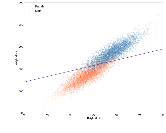
Now we can use the coefficients to plot a separating line in height-weight space.

logit_pars = male_logit.params
intercept = -logit_pars['Intercept'] / logit_pars['Weight']
slope = -logit_pars['Height'] / logit_pars['Weight']

Let’s plot the data, color-coded by sex, and the separating line.

fig = plt.figure(figsize = (10, 8))
# Women points (coral)
plt.plot(heights_f, weights_f, '.', label = 'Female',
mfc = 'None', mec='coral', alpha = .4)
# Men points (blue)
plt.plot(heights_m, weights_m, '.', label = 'Male',
mfc = 'None', mec='steelblue', alpha = .4)
# The separating line
plt.plot(array([50, 80]), intercept + slope * array([50, 80]),
'-', color = '#461B7E')
plt.xlabel('Height (in.)')
plt.ylabel('Weight (lbs.)')
plt.legend(loc='upper left')

Conclusion

There are several more examples using Patsy formulas with statsmodels functions in later chapters. If you’re accustomed to R’s formula notation, the transition from running models in R to running models in statsmodels is easy. One of the annoying things in Python versus R is the need to pull arrays out of pandas dataframes, because the functions you want to apply to the data (say estimating models, or plotting) don’t interface with the dataframe, but instead numpy arrays. It’s not terrible, but it adds a layer of friction in the analysis. So it’s great that statsmodels is starting to integrate well with pandas.